I have just filed a new PR which adds Naive Bayes Classifiers to rusty-machine. I thought it would be fun to talk through some of the process I undertook whilst creating this model.
The contents of the post will be loosely broken up as follows:
- What is a Naive Bayes Classifier?
- Design
- Implementing the rusty-machine traits
- Writing the model code
- Testing
- What’s missing?
This is a pretty long post which attempts to cover the end-to-end process of implementing a machine learning model in rusty-machine. Note that the implementation of Naive Bayes described here may change.
Naive Bayes Classifiers
Naive Bayes Classifiers are a very simple but effective classification model. They provide a probabilistic model that separates out our data into classes. I wont dig too much into the maths (there are plenty of resources online) but will include a rough overview.
The model treats each input vector as a number of statistically independent features. Each class within the model represents a distribution for a collection of these vectors. When training we are computing the distribution for each class based on our input data. When testing we are finding the class which the data is most likely to belong to.
Using the independence assumption and Bayes’ rule we can compute the distribution for the classes easily.
Designing this model in Rust
When designing models in rusty-machine the question I tend to focus on is how flexible should we be? We want the model to be easy to use - hiding as much of the nitty-gritty from our user as possible. However, advanced users may want to make use of this stuff and even extend it for their own purposes. Additionally with many models, including Naive Bayes, we have different variants. For Naive Bayes this means different underlying class distributions - we should support these too.
Rusty-machine provides some traits for models which we use to create a consistent API. In the case of Naive Bayes, a Supervised learning algorithm, we want the SupModel trait. We should implement this trait for our NaiveBayes struct.
As for distributions we should also provide a trait here - which I decided to name Distribution. This trait provides functions which will be utilized by the Naive Bayes model when it is using the distribution.
The aspect of design which I spent the most time trying to figure out was where the split between model logic and distribution logic should occur. This is something which even now I think I haven’t quite got right. We want the model to handle as much as possible so that is easy for users to implement new Distributions. However, we also need to worry about performance - computing probabilities is going to be intense for some models and will be solved in different ways for each distribution. We also want the user to be able to tweak the distribution in various ways. Sadly this last point is largely inaccessible in the current design.
That was all very abstract… I’m sorry if it doesn’t make sense. In the next sections we’ll be looking at some real code samples which will hopefully illuminate how the above discussion comes into play.
Implementing the rusty-machine traits
We have our Naive Bayes model which looks like this:
/// The Naive Bayes model.
pub struct NaiveBayes<T: Distribution> {
    distr: Option<T>,
    cluster_count: Option<usize>,
    class_prior: Option<Vec<f64>>,
    class_counts: Vec<usize>,
}
It specifies a distribution and some other data which will be filled during training. Now we need to implement the traits and the model logic. The first trait mentioned above was SupModel:
/// Trait for supervised model.
pub trait SupModel<T,U> {

    /// Predict output from inputs.
    fn predict(&self, inputs: &T) -> U;

    /// Train the model using inputs and targets.
    fn train(&mut self, inputs: &T, targets: &U);
}
This trait provides the interface for supervised models. In our Naive Bayes model training looks like this:
/// Train the model using inputs and targets.
fn train(&mut self, inputs: &Matrix<f64>, targets: &Matrix<f64>) {
    self.distr = Some(T::from_model_params(targets.cols(), inputs.cols()));
    self.update_params(inputs, targets);
}
Here we instantiate our distribution with the class and feature counts. We then update the parameters of the distribution using the input and target data. The predict trait is fairly simple too:
/// Predict output from inputs.
fn predict(&self, inputs: &Matrix<f64>) -> Matrix<f64> {
    let log_probs = self.get_log_probs(inputs);
    let input_classes = NaiveBayes::<T>::get_classes(log_probs);

    // We convert the classes into our output format
}
The first line computes the log-probability that each input lies within a class. The second line argmax’s this matrix to get the class that the input is most likely to belong to. There is a little more code in this method which massages the input_classes into our output format.
Next up is the Distribution trait which is implemented by the distr field in the NaiveBayes model. This trait looks like this:
/// Naive Bayes Distribution.
pub trait Distribution {
    /// Initialize the distribution parameters.
    fn from_model_params(class_count: usize, features: usize) -> Self;

    /// Updates the distribution parameters.
    fn update_params(&mut self, data: Matrix<f64>, class: usize);

    /// Compute the joint log likelihood of the data.
    ///
    /// Returns a matrix with rows containing the probability that the input lies in each class.
    fn joint_log_lik(&self, data: &Matrix<f64>, class_prior: &[f64]) -> Matrix<f64>;
}
This trait allows us to create a new Distribution with the correct size parameters. The update_params function is used when training the model and joint_log_lik during testing.
This format makes it fairly easy for a user to add a new Distribution if they wanted to. Most of the heavy lifting for the naive Bayes model happens within the distribution - this was primarily to allow control over the probability computation.
Writing the model code
After implementing our distributions we don’t have too much more work within the model.
For training the logic is almost entirely contained in the distributions. We need to compute the class_priors but this is a fairly simple addition.
For predicting we only have a little more to do. Once we get the log-probabilities from the distribution we argmax each row to find the most likely class for each input.
Testing
I wanted to include this section as it isn’t immediately obvious how we should test that our machine learning algorithms work correctly.
We want to ensure that each of our proposed Distributions works correctly. There are a couple of ways we can do this.
Simple testing
One simple test is to make some dummy data that has some clear class structure. For example for our Gaussian model we may take:
⎡1.0,1.1,1.2⎤ - Class 1
⎢0.9,1.3,1.1⎥ - Class 1
⎢6.9,5.3,5.5⎥ - Class 2
⎣5.5,7.0,6.0⎦ - Class 2
Here we can see a pretty clear distinction between data in class 1 and class 2 - the former having smaller feature values. We can feed the model this data and see if it can correctly predict the same training inputs. We can also manually inspect the distribution to confirm it looks sensible.
More advanced testing
An obvious and great way to test is to pick some real world data! UC Irvine have a large collection of open source data sets we can try new models out on.
Another technique that is particularly well suited to probabilistic models like Naive Bayes, is to generate data from a sample model and try to learn what the parameters of the sample model were. I’ll run through a simple example below.
Let’s once again take the Gaussian Naive Bayes model as our example. Suppose we have two classes and a two-dimensional feature space. We need to pick a mean and variance (μ, σ2) for each feature in both classes - 8 values in total.
Once we have chosen these values we sample from the respective distributions - our samples may look like this:
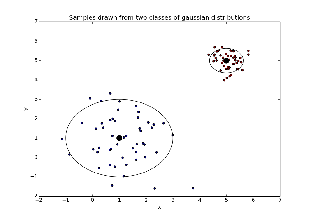 In the above the class means are shown as black dots with the smaller dots around them being the samples. The larger rings represent the variance of the distributions*.
We feed these samples into our model with the respective classes that they came from. The hope is that we can recover the values we chose initially.
* The ring is a 95% confidence interval about the mean. I thought the ring would be prettier than a box showing the variance…
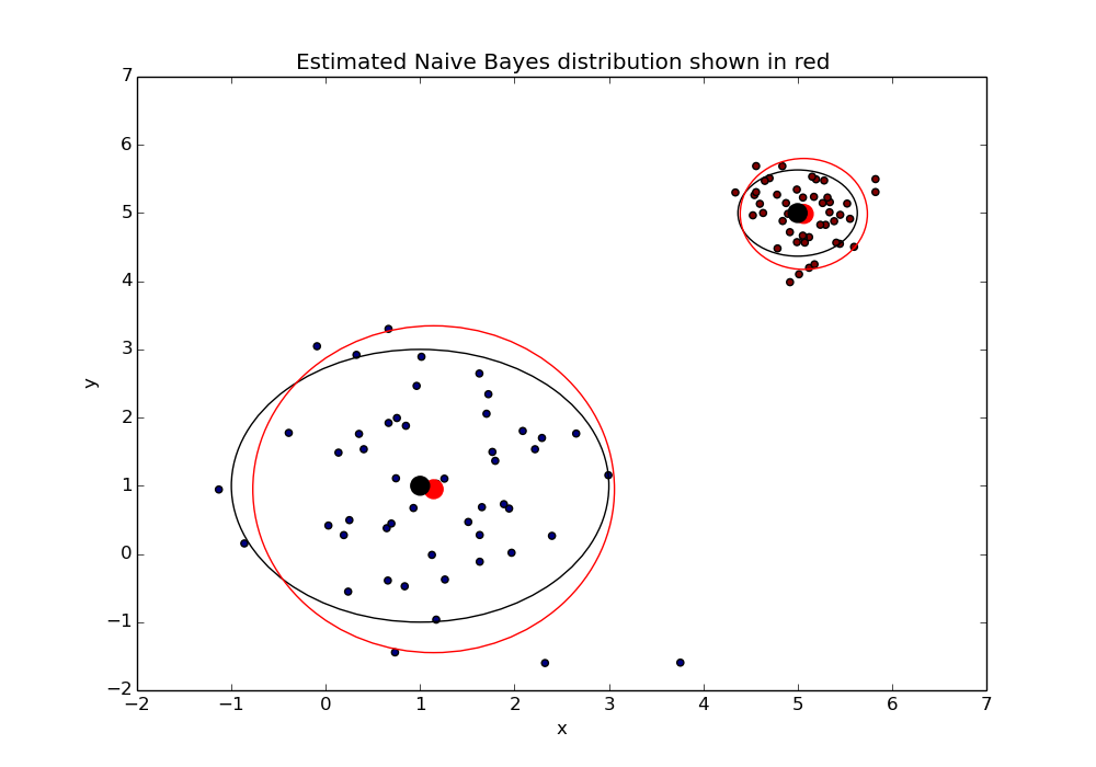
Great! Looks like our model can correctly infer the original distribution. This gives us a pretty good sense that our model is working correctly.
Of course even if all the above tests look good it doesn’t mean that our model is perfect and ready to solve any classification problem. We can only safely say that our model does well when the data fits the model’s assumptions. Luckily in practice Naive Bayes does surprisingly well despite it’s strong assumptions.
What’s missing?
Checking model inputs.
We should ensure that the inputs to the model conform to the expected shape. Or perhaps broadcast them into the correct shape. Though this is an issue with all the current models.
Allowing specification of pseudo counts on the discrete models.
This is not currently supported and pseudo count is simply defaulted to 1. This is a pretty minor point but it would be good to provide this access in general.
Partial training (so we can go in batches).
This would be a nice addition and is possible in the current scope. I will hopefully add this in the future.
Optimal code.
There are a few inefficient areas. Stemming from both the linear algebra library and the interface design. Similar work will need to be done across all models in the future.
Closing Remarks
As always I’d really appreciate feedback on this post, rusty-machine, my implementation of Naive Bayes and just about anything else related.
Rusty-machine can always use more contributors and there are a range of skills needed (it’s not all machine learning - though there’s definitely the opportunity to learn that if you’re interested). Thank you to those who are currently working on the library; danlrobertson, zackmdavis and others!